Simulating trades with order flow triggers

A trading algorithm that looks at historical data and outputs a dataframe of trades.

Report Bug · Request Feature

About The Project

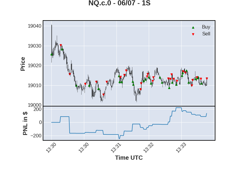
This code analyzes trading activity among the 100 stocks that comprise the Nasdaq 100, and creates a dataframe of trades based on NQ bid/ask. This dataframe is then overlayed on a Candlestick chart.

Built With

• 
• 
• 
• 
• 
• 

Getting Started

Requirements

• To run the Jupyter notebook, you'll need an appropriate environment. I'm using Visual Studio Code with the Jupyter extension.
• You will need an API key from Databento.
• You will need Python installed.

Installation

• Clone the repo

  git clone https://github.com/gty3/python_nq.git

• Open the project with your choice of Jupyter platform.

• Rename env.example to .env and add your DATABENTO_API_KEY

• Open main.ipynb and select Run All.

Usage

The project is divided into 4 cells.

Cell 1 imports 3 datasets using the get_range method:

• The first 2 datasets use the "tbbo" schema - "Top of Book Bid and Offer". While the order book data is necessary for logging the NQ trade prices, it is not necessary for the underlying instruments orders. However, as these datasets are merged, it enables more concise code.
• The 3rd dataset uses the "ohlcv-1s" schema to create our Candlestick chart in cell 4.

Cell 2 implements the trading logic for the algorithm. It aggregates the number of buys and sells across the 100 underlying instruments each second.

• If the trade condition is met, log the nq bid/ask price in the trades dataframe.
• The modify_trades function removes trades that do not conform to one contract open.
• The calculate_pnl function adds a current trade and total profit & loss.

Cell 3 uses dtale to view the trades dataframe. This is a great tool to visualize the dataframe while modifying the code.

Cell 4 creates a Candlestick chart using mplfinance. The trades dataframe is seperated into two, buy and sell dataframes, which are overlayed on a Candlestick chart plotted from the OHLCV data.

Making Changes

You can change the instruments being traded by altering the variables ‘symbols’ and ‘dataset’, as well as the instruments that are monitored with ‘underlying_symbols’ and ‘underlying_dataset’. It works for both stocks and futures. For more information on the available symbols and datasets - https://databento.com/docs/api-reference-historical/basics/datasets

Change the trade conditions by modifying the ‘create_trades_df’ in /trade_utils.py. Change the multiplier or invert the condtion '>' or '<'.

buy_condition = (grouped_df['underlying_total_sells'] > grouped_df['underlying_total_buys'] * 2)

Modify 'group_and_aggregate' in /trade_utils.py to change the condition's attributes. For example change 'underlying_total_sells' to the attribute underlying_sells_average=('side', lambdax: x.eq('A').mean())

Changing the time frame of the trade condition requires modifying the chart time frame as well. In order for the trades to overlay on the Candlestick plot, the trades dataframe keys need to match Candlestick dataframe keys.

Roadmap

• Simulate network latency.
• Add a stop loss.
• Add max duration to a trade.
• Use live data.

License

Distributed under the MIT License. See LICENSE.txt for more information.

Contact

Geoff Young - @gty_

Project Link: https://github.com/gty3/python_nq